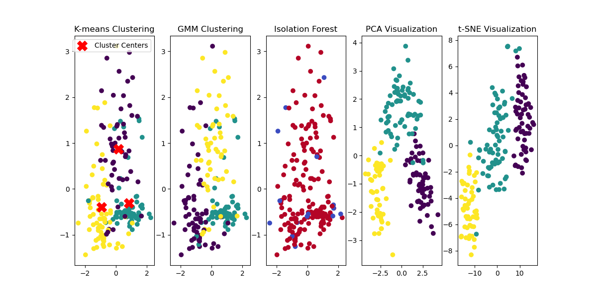
Project 2: Comparison unsupervised models

Comparison unsupervised models

The "load_wine" dataset is a built-in dataset in scikit-learn that contains information about wines. It is often used for classification tasks, where the goal is to predict the class of a wine based on its attributes. However, the dataset can be adapted for clustering and other unsupervised learning tasks as well.

To compare the different algorithms (clustering, biclustering, Gaussian Mixture Model, Isolation Forest, manifold learning, and Principal Component Analysis) on this dataset, we first need to modify the dataset to suit each task accordingly. Keep in mind that the suitability of each algorithm can depend on the specific characteristics of the dataset and the nature of the problem at hand.

Let's go through each algorithm and its potential application to this dataset:

1. Clustering Algorithms (e.g., K-means, Hierarchical Clustering):

Clustering algorithms group data points into clusters based on similarity. This can be useful if we want to discover inherent patterns or subgroups within the wine data. However, it's worth noting that for clustering, we usually do not have labeled data, so we will be using unsupervised techniques.

2. Biclustering Algorithms (e.g., Spectral Co-clustering, Biclustering):

Biclustering algorithms simultaneously cluster both rows and columns of a dataset. If there are specific patterns where some wines have similar attributes across specific features, biclustering might be useful to identify these patterns.

3. Gaussian Mixture Model (GMM):

GMM is a probabilistic model that can assign probabilities of data points belonging to different clusters. It assumes that the data is generated from a mixture of several Gaussian distributions. GMM can be useful if we have overlapping clusters in the wine dataset and want to assign probabilities of data points belonging to different wine types.

4. Isolation Forest:

Isolation Forest is an anomaly detection algorithm that identifies outliers or anomalies in the data. If there are some wines in the dataset that are very different from the majority, Isolation Forest can help identify them.

5. Manifold Learning (e.g., t-SNE, UMAP):

Manifold learning algorithms aim to reduce the dimensionality of the data while preserving the underlying structure. If the wine dataset has a high number of features and we want to visualize or analyze it in a lower-dimensional space, manifold learning can be useful.

6. Principal Component Analysis (PCA):

PCA is another dimensionality reduction technique that transforms data into a new coordinate system representing the principal components of the data. It can be useful to reduce the number of features and extract the most important ones for the wine dataset.

Now, to determine which algorithm is most appropriate for this dataset, we need to consider the characteristics of the data and the specific goals of the analysis:

- If we want to explore inherent patterns and subgroups within the wine data, clustering algorithms could be a good fit.

- If there are specific patterns where some wines have similar attributes across certain features, biclustering might be helpful.

- If there is a possibility of overlapping clusters, Gaussian Mixture Model could be appropriate.

- For anomaly detection and identifying outlying wines, Isolation Forest can be useful.

- If we want to visualize the data in a lower-dimensional space, manifold learning algorithms like t-SNE or UMAP can be helpful.

- To extract important features and reduce dimensionality, PCA is a classic choice.

Ultimately, the most appropriate algorithm depends on the specific insights or goals you want to achieve with the wine dataset. It is recommended to try out multiple algorithms and evaluate their results using appropriate metrics (e.g., silhouette score for clustering, reconstruction error for dimensionality reduction) to make an informed decision. Also, preprocessing the data, handling missing values, and scaling the features could impact the performance of the algorithms, so those steps should not be overlooked.

Results

Below is a brief example of how you can start comparing some of these algorithms using scikit-learn in Python:


import numpy as np
from sklearn.datasets import load_wine
from sklearn.preprocessing import StandardScaler
from sklearn.cluster import KMeans
from sklearn.mixture import GaussianMixture
from sklearn.decomposition import PCA
from sklearn.manifold import TSNE
from sklearn.ensemble import IsolationForest
from sklearn.metrics import silhouette_score
import matplotlib.pyplot as plt

# Load the wine dataset
data = load_wine()
X, y = data.data, data.target

# Standardize the features
scaler = StandardScaler()
X_scaled = scaler.fit_transform(X)

# Apply different algorithms
# Clustering - K-means
kmeans = KMeans(n_clusters=3, random_state=42)
kmeans_labels = kmeans.fit_predict(X_scaled)
kmeans_silhouette = silhouette_score(X_scaled, kmeans_labels)

# Gaussian Mixture Model
gmm = GaussianMixture(n_components=3, random_state=42)
gmm_labels = gmm.fit_predict(X_scaled)
gmm_silhouette = silhouette_score(X_scaled, gmm_labels)

# Principal Component Analysis (PCA)
pca = PCA(n_components=2, random_state=42)
X_pca = pca.fit_transform(X_scaled)

# t-SNE for visualization
tsne = TSNE(n_components=2, random_state=42)
X_tsne = tsne.fit_transform(X_scaled)

# Isolation Forest for anomaly detection
iso_forest = IsolationForest(random_state=42)
is_outlier = iso_forest.fit_predict(X_scaled)
num_outliers = np.sum(is_outlier == -1)

# Plot clustering results
plt.figure(figsize=(12, 6))
plt.subplot(1, 5, 1)
plt.scatter(X_scaled[:, 0], X_scaled[:, 1], c=kmeans_labels, cmap='viridis')
plt.scatter(kmeans.cluster_centers_[:, 0], kmeans.cluster_centers_[:, 1], s=200, c='red', marker='X', label='Cluster Centers')
plt.title('K-means Clustering')
plt.legend()

plt.subplot(1, 5, 2)
plt.scatter(X_scaled[:, 0], X_scaled[:, 1], c=gmm_labels, cmap='viridis')
plt.title('GMM Clustering')

plt.subplot(1, 5, 3)
plt.scatter(X_scaled[:, 0], X_scaled[:, 1], c=is_outlier, cmap='coolwarm') # (Outliers in Blue)
plt.title('Isolation Forest')

plt.subplot(1, 5, 4)
plt.scatter(X_pca[:, 0], X_pca[:, 1], c=y, cmap='viridis')
plt.title('PCA Visualization')

plt.subplot(1, 5, 5)
plt.scatter(X_tsne[:, 0], X_tsne[:, 1], c=y, cmap='viridis')
plt.title('t-SNE Visualization')
plt.show()

# Print evaluation metrics
print(f"K-means Silhouette Score: {kmeans_silhouette:.4f}")
print(f"GMM Silhouette Score: {gmm_silhouette:.4f}")
print(f"Number of Outliers (Isolation Forest): {num_outliers}")

K-means Silhouette Score: 0.2849
GMM Silhouette Score: 0.2844
Number of Outliers (Isolation Forest): 15