Manifold Learning

Manifold learning is a concept in machine learning that helps us understand and visualize complex data in simpler ways. Imagine you have a bunch of data points in a high-dimensional space, like points scattered across multiple dimensions. It's difficult to visualize or make sense of this data directly.

Manifold learning aims to find a lower-dimensional representation or structure hidden within this high-dimensional data. It assumes that the data points lie on or near a lower-dimensional manifold, which is like a curved sheet or surface embedded in the high-dimensional space. The manifold captures the essential structure and relationships between the data points.

The goal of manifold learning algorithms is to unfold or unroll this curved sheet in a way that preserves the relationships between the data points. It tries to find a lower-dimensional representation where the data points maintain their relative positions and distances as much as possible.

By reducing the dimensionality, manifold learning can help us visualize and understand the data better. It can reveal patterns, clusters, or other structures that are not easily visible in the original high-dimensional space. This lower-dimensional representation can also be used for other machine learning tasks like classification or regression.

In simpler terms, manifold learning helps us simplify and make sense of complex data by finding a lower-dimensional structure hidden within it. It's like unfolding a crumpled piece of paper to reveal its original shape, allowing us to understand the relationships between the data points more easily.
Python Example

Let's consider an example using the popular manifold learning algorithm called t-SNE (t-Distributed Stochastic Neighbor Embedding) in Python. We'll use the scikit-learn library, which provides various machine learning algorithms, including manifold learning techniques.

import numpy as np
import matplotlib.pyplot as plt
from sklearn.manifold import TSNE

# Generate some random high-dimensional data
np.random.seed(42)
n_samples = 100
n_features = 50
X = np.random.rand(n_samples, n_features)

# Perform t-SNE to obtain the lower-dimensional representation
tsne = TSNE(n_components=2)
X_tsne = tsne.fit_transform(X)

# Plot the results
plt.scatter(X_tsne[:, 0], X_tsne[:, 1])
plt.title("t-SNE Visualization")
plt.xlabel("Component 1")
plt.ylabel("Component 2")
plt.show()

Results:

In this example, we generate random high-dimensional data using NumPy. Then, we use the TSNE class from scikit-learn to create a t-SNE object. We specify n_components=2 to obtain a 2-dimensional representation.

Next, we call the fit_transform() method on the t-SNE object, passing in our high-dimensional data X. This step performs the t-SNE algorithm and returns the lower-dimensional representation X_tsne.

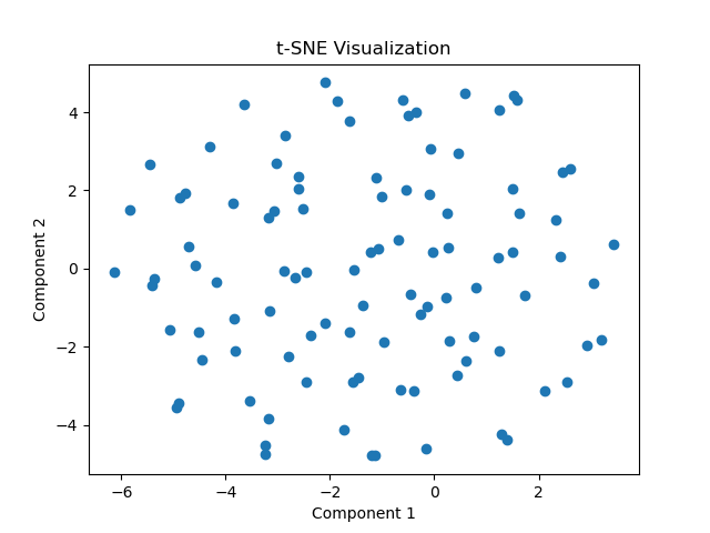
Finally, we plot the resulting 2-dimensional representation using Matplotlib. Each point in the plot corresponds to a data point in the original high-dimensional space. The plot allows us to visualize the data in a simplified form, where the relative positions of the points reflect their relationships in the high-dimensional space.

Note that the t-SNE algorithm is stochastic, meaning it can produce different results with each run. You may need to experiment with different settings, such as the perplexity parameter, to achieve optimal visualizations for your specific data.