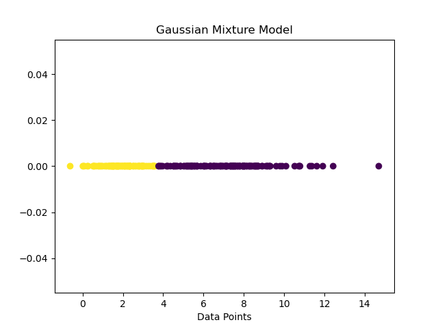
Gaussian Mixture

Imagine you have a group of data points that you want to analyze. Each data point represents something, like the height of people or the scores of students in a test. Now, you suspect that the data points might come from different groups or categories. For example, in the case of height, there might be one group of short people and another group of tall people.

A Gaussian Mixture Model (GMM) helps us identify and understand these underlying groups or categories within our data. It assumes that each group is represented by a bell-shaped curve, called a Gaussian distribution or a normal distribution. A Gaussian distribution is defined by its average value (mean) and how spread out it is (standard deviation).

The GMM combines multiple Gaussian distributions to create a mixture model. It assumes that our data points are generated by these individual Gaussian distributions with different means and standard deviations. The mixture model combines these distributions in a way that allows us to capture the characteristics of each group within our data.

To find the best fit for our data, the GMM uses an iterative process called the Expectation-Maximization (EM) algorithm. This algorithm calculates the probability that each data point belongs to each group and adjusts the parameters (mean and standard deviation) of the Gaussian distributions to maximize the likelihood of the observed data.

In simpler terms, a Gaussian Mixture Model helps us identify groups within our data by fitting multiple bell-shaped curves to the data and adjusting them until they best represent the underlying patterns. It's like finding different categories in a dataset based on their distribution patterns.

Python Example

import numpy as np
import matplotlib.pyplot as plt
from sklearn.mixture import GaussianMixture

# Generating synthetic data
np.random.seed(42)
# Data points from the first group (mean: 2, standard deviation: 1)
data1 = np.random.normal(loc=2, scale=1, size=100)
# Data points from the second group (mean: 7, standard deviation: 2)
data2 = np.random.normal(loc=7, scale=2, size=150)
# Combining the two groups
data = np.concatenate([data1, data2])

# Fitting the Gaussian Mixture Model
gmm = GaussianMixture(n_components=2)  # We assume there are two groups
gmm.fit(data.reshape(-1, 1))

# Predicting the group labels for each data point
labels = gmm.predict(data.reshape(-1, 1))

# Plotting the data points and their assigned labels
plt.scatter(data, np.zeros_like(data), c=labels, cmap='viridis')
plt.title('Gaussian Mixture Model')
plt.xlabel('Data Points')
plt.show()

Results:

In this example, we generate synthetic data with two underlying groups. We use the numpy library to generate random data points from two normal distributions. Then, we concatenate the two groups to create our dataset.

Next, we use the GaussianMixture class from scikit-learn to fit the GMM to our data. We set n_components=2 to indicate that we expect two underlying groups.

After fitting the GMM, we predict the group labels for each data point using the predict method. Finally, we visualize the data points and their assigned labels using a scatter plot.

The resulting plot should show the two groups with different colors, representing the separation of the data points into the identified clusters by the GMM.