Gaussian Process

The Gaussian process algorithm is a machine learning technique that allows us to make predictions and estimate uncertainty in a flexible and powerful way.

Imagine you have a set of data points, and you want to understand the underlying pattern or relationship between them. The Gaussian process algorithm helps us do that by assuming that the data points are drawn from a distribution called a Gaussian process.

In simpler terms, a Gaussian process is like a collection of infinitely many random variables, where each variable represents the value of a data point at a particular location. The interesting thing is that the values of these variables are not entirely random. Instead, they follow a pattern or a smooth curve.

With a Gaussian process, we start by assuming a certain shape or form for this curve. Then, based on the data we have, the algorithm calculates the probability of different curves that could explain the data. It considers both the similarity of the observed data points and the uncertainty in the predictions.

The algorithm essentially creates a distribution of possible curves, with the most likely curve being the one that fits the data points the best. This distribution gives us not only the predicted values for new data points but also a measure of uncertainty or confidence in those predictions.

So, to summarize, the Gaussian process algorithm helps us understand the relationship between data points by assuming a smooth curve and estimating the uncertainty in our predictions. It's a flexible and powerful tool for making predictions and understanding patterns in various fields like machine learning, statistics, and optimization.
Python Example

import numpy as np
import matplotlib.pyplot as plt
from sklearn.gaussian_process import GaussianProcessRegressor
from sklearn.gaussian_process.kernels import RBF, WhiteKernel

# Generate synthetic data
np.random.seed(0)
X = np.random.rand(20, 1) * 10
y = np.sin(X) + 0.1 * np.random.randn(20, 1)

# Define the kernel for the Gaussian process
kernel = 1.0 * RBF(length_scale=1e1, length_scale_bounds=(1e-2, 1e3)) + WhiteKernel(
    noise_level=1, noise_level_bounds=(1e-5, 1e1)
)

# Create a Gaussian process regressor
gp = GaussianProcessRegressor(kernel=kernel)

# Fit the Gaussian process model to the data
gp.fit(X, y)

# Generate test data
X_test = np.linspace(0, 10, 100).reshape(-1, 1)

# Make predictions with the Gaussian process model
y_pred, y_std = gp.predict(X_test, return_std=True)

# Plot the results
plt.figure(figsize=(10, 6))
plt.scatter(X, y, color='blue', label='Observations')
plt.plot(X_test, y_pred, color='red', label='Predicted Values')
plt.fill_between(X_test.squeeze(), (y_pred - 2 * y_std).squeeze(), (y_pred + 2 * y_std).squeeze(),
          color='gray', alpha=0.3, label='Uncertainty')
plt.xlabel('X')
plt.ylabel('y')
plt.title('Gaussian Process Regression')
plt.legend()
plt.show()

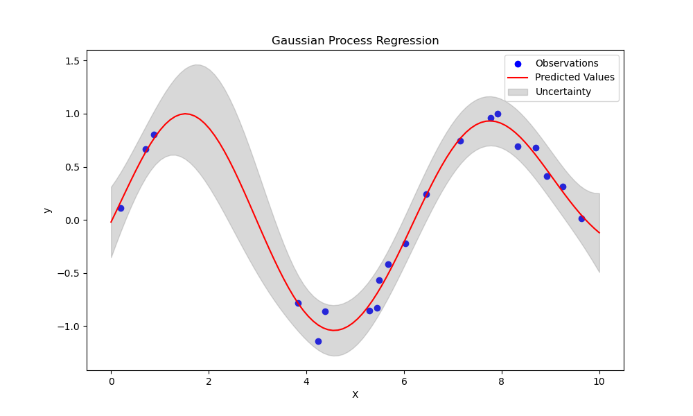
Results:

In this example, we first generate some synthetic data points X and corresponding target values y. We assume a sine function with some random noise.

Next, we define the kernel for the Gaussian process. In this case, we use the Radial Basis Function (RBF) kernel, which is commonly used for smooth functions.

Then, we create an instance of GaussianProcessRegressor and fit the model to our data.

After that, we generate some test data X_test to make predictions on. We use the predict method of the Gaussian process model to obtain the predicted values y_pred and the standard deviation y_std as measures of uncertainty.

This is a basic example to help you understand the usage of Gaussian process regression in Python. The scikit-learn library provides more advanced functionalities and options for customization.